Modelling Motivation#

This notebook can be directly downloaded here to run it locally.

Simulation of a corridor with different motivations#

In this demonstration, we model a narrow corridor scenario featuring three distinct groups of agents. Among them, one group exhibits a higher level of motivation compared to the others.

We employ the collision-free speed model to determine the speed of each agent. This speed is influenced by the desired speed, denoted as \(v^0\), the agent’s radius \(r\), and the slope factor \(T\).

The varying motivation levels among the groups are represented by different \(T\) values. The rationale for using \(T\) to depict motivation is that highly motivated pedestrians, who are more aggressive in their movements, will quickly occupy any available space between them, correlating to a lower \(T\) value. Conversely, less motivated pedestrians maintain a distance based on their walking speed, aligning with a higher \(T\) value.

To accentuate this dynamic, the first group of agents will decelerate a few seconds into the simulation. As a result, we’ll notice that the second group, driven by high motivation, will swiftly close distances and overtake the first group as it reduces speed. In contrast, the third group, with average motivation, will decelerate upon nearing the slower agents, without attempting to pass them.

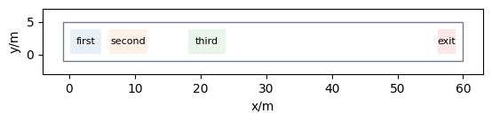
Setting up the geometry#

We will be using the a corridor 40 meters long and 4 meters wide.

corridor = [(-1, -1), (60, -1), (60, 5), (-1, 5)]

areas = {}
areas["first"] = Polygon([[0, 0], [5, 0], [5, 4], [0, 4]])
areas["second"] = Polygon([[6, 0], [12, 0], [12, 4], [6, 4]])
areas["third"] = Polygon([[18, 0], [24, 0], [24, 4], [18, 4]])
areas["exit"] = Polygon([(56, 0), (59, 0), (59, 4), (56, 4)])

walkable_area = pedpy.WalkableArea(corridor)

../_images/984a34dcbcbc3b8cc91681ba88b93e69f65276c1dd6d1f7c63a9fef22300717d.png

Operational model#

Now that the geometry is set, our subsequent task is to specify the model and its associated parameters.
For this demonstration, we’ll employ the “collision-free” model.
However, since we are interested in two different motivation states, we will have to define two different time gaps.

T_normal = 1.3
T_motivation = 0.1
v0_normal = 1.5
v0_slow = 0.5

Note, that in JuPedSim the model parameter \(T\) is called time_gap.

The values \(1.3\, s\) and \(0.1\, s\) are chosen according to the paper Rzezonka2022, Fig.5.

Setting Up the Simulation Object#

Having established the model and geometry details, and combined with other parameters such as the time step \(dt\), we can proceed to construct our simulation object as illustrated below:

trajectory_file = "trajectories.sqlite"
simulation = jps.Simulation(
    dt=0.05,
    model=jps.CollisionFreeSpeedModel(
        strength_neighbor_repulsion=2.6,
        range_neighbor_repulsion=0.1,
        range_geometry_repulsion=0.05,
    ),
    geometry=walkable_area.polygon,
    trajectory_writer=jps.SqliteTrajectoryWriter(
        output_file=pathlib.Path(trajectory_file)
    ),
)

Specifying Routing Details#

At this point, we’ll provide basic routing instructions, guiding the agents to progress towards an exit point, which is in this case at the end of the corridor.

exit_id = simulation.add_exit_stage(areas["exit"])
journey_id = simulation.add_journey(jps.JourneyDescription([exit_id]))

Defining and Distributing Agents#

Now, we’ll position the agents and establish their attributes, leveraging previously mentioned parameters. We will distribute three different groups in three different areas.

First area contains normally motivated agents.
The second area contains motivated agents that are more likely to close gaps to each other.
The third area contains normally motivated agents. These agents will reduce their desired speeds after some seconds.

Distribute normal agents in the first area#

total_agents_normal = 20
positions = jps.distribute_by_number(
    polygon=Polygon(areas["first"]),
    number_of_agents=total_agents_normal,
    distance_to_agents=0.4,
    distance_to_polygon=0.4,
    seed=45131502,
)

for position in positions:
    simulation.add_agent(
        jps.CollisionFreeSpeedModelAgentParameters(
            position=position,
            v0=v0_normal,
            time_gap=T_normal,
            journey_id=journey_id,
            stage_id=exit_id,
        )
    )

Distribute motivated agents in the second area#

total_agents_motivated = 20
positions = jps.distribute_by_number(
    polygon=Polygon(areas["second"]),
    number_of_agents=total_agents_motivated,
    distance_to_agents=0.6,
    distance_to_polygon=0.6,
    seed=45131502,
)
for position in positions:
    simulation.add_agent(
        jps.CollisionFreeSpeedModelAgentParameters(
            position=position,
            v0=v0_normal,
            time_gap=T_motivation,
            journey_id=journey_id,
            stage_id=exit_id,
        )
    )

Distribute normal agents in the third area#

total_agents_motivated_delay = 20
positions = jps.distribute_by_number(
    polygon=Polygon(areas["third"]),
    number_of_agents=total_agents_motivated_delay,
    distance_to_agents=0.8,
    distance_to_polygon=0.4,
    seed=45131502,
)
ids_third_group = set(
    [
        simulation.add_agent(
            jps.CollisionFreeSpeedModelAgentParameters(
                position=position,
                v0=v0_normal,
                time_gap=T_normal,
                journey_id=journey_id,
                stage_id=exit_id,
            )
        )
        for position in positions
    ]
)

Executing the Simulation#

With all components in place, we’re set to initiate the simulation. For this demonstration, the trajectories will be recorded in an sqlite database.

simulation.iterate(200)
for id in ids_third_group:
    for agent in simulation.agents():
        if agent.id == id:
            agent.model.v0 = v0_slow

while simulation.agent_count() > 0:
    simulation.iterate()

Visualizing the Trajectories#

For trajectory visualization, we’ll extract data from the sqlite database. A straightforward method for this is employing the jupedsim-visualizer.

from jupedsim.internal.notebook_utils import animate, read_sqlite_file

agent_trajectories, walkable_area = read_sqlite_file(trajectory_file)
animate(
    agent_trajectories,
    walkable_area,
    every_nth_frame=5,
    width=1000,
    height=500,
)

Notes and Comments#

It’s noticeable that members of the second group tend to draw nearer to each other compared to those in the first group, primarily attributed to their lower \(T\) values. As the third group begins to decelerate after a while, due to an adjustment in the target speed \(v_0\), the second group seizes this opportunity to bridge the distance and surpass them.

Conversely, the first group maintains a consistent pace and doesn’t attempt to overtake the now-lagging third group.

Download#