Movement through Bottlenecks#

This notebook can be directly downloaded here to run it locally.

In this following, we’ll investigate the movement of a crowd through two successive bottlenecks with a simulation. We expect that a jam occurs at the first bottleneck but not at the second one since the flow is considerably reduced by the first bottleneck.

For this purpose, we’ll setup a simulation scenario according to the RiMEA Test 12 [1] and analyse the results with pedpy to inspect the density and flow. After that we’ll vary the width of the bottlenecks and investigate the effects on the movement.

Let’s begin by importing the required packages for our simulation:

import pathlib

import jupedsim as jps
import matplotlib.pyplot as plt
import pandas as pd
import pedpy
from numpy.random import normal  # normal distribution of free movement speed
from shapely import GeometryCollection, Polygon

Geometry Setup#

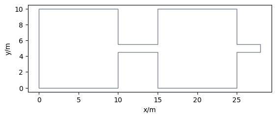
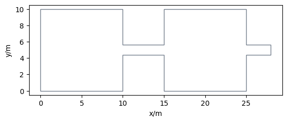
Let’s construct the geometry according to RiMEA by defining two rooms and a corridor with a width of 1 meter. To consider the interactions of agents in the second bottleneck (when leaving the second room) the corridor ends 3 meters behind the second room. By creating the union of all parts we end up with the whole walkable area.

room1 = Polygon([(0, 0), (10, 0), (10, 10), (0, 10)])
room2 = Polygon([(15, 0), (25, 0), (25, 10), (15, 10)])
corridor = Polygon([(10, 4.5), (28, 4.5), (28, 5.5), (10, 5.5)])

area = GeometryCollection(corridor.union(room1.union(room2)))
walkable_area = pedpy.WalkableArea(area.geoms[0])
pedpy.plot_walkable_area(walkable_area=walkable_area).set_aspect("equal")

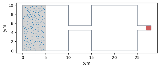
../_images/32b1d7b60d758c3254f06aac9d27f7c181059a82943664b543beb4b03090818c.png

Definition of Start Positions and Exit#

Now we define the spawning area according to RiMEA and calculate 150 positions within that area. The exit area is defined at the end of the corridor.

spawning_area = Polygon([(0, 0), (5, 0), (5, 10), (0, 10)])
num_agents = 150
pos_in_spawning_area = jps.distributions.distribute_by_number(
    polygon=spawning_area,
    number_of_agents=num_agents,
    distance_to_agents=0.3,
    distance_to_polygon=0.15,
    seed=1,
)
exit_area = Polygon([(27, 4.5), (28, 4.5), (28, 5.5), (27, 5.5)])

Let’s have a look at our setup:

plot_simulation_configuration(
    walkable_area, spawning_area, pos_in_spawning_area, exit_area
)

../_images/b22b3b91a4d2502f55c1829f31a38f52ef3e06b312409312c8a349f5ffd86acf.png

Specification of Parameters und Running the Simulation#

Now we just need to define the details of the operational model, routing and the specific agent parameters. In this example, the agents share the same parameters, ecxept for their free movement speed (and starting position).

trajectory_file = "double-botteleneck.sqlite"  # output file
simulation = jps.Simulation(
    model=jps.CollisionFreeSpeedModel(),
    geometry=area,
    trajectory_writer=jps.SqliteTrajectoryWriter(
        output_file=pathlib.Path(trajectory_file)
    ),
)

exit_id = simulation.add_exit_stage(exit_area.exterior.coords[:-1])
journey = jps.JourneyDescription([exit_id])
journey_id = simulation.add_journey(journey)

v_distribution = normal(1.34, 0.05, num_agents)

for pos, v0 in zip(pos_in_spawning_area, v_distribution):
    simulation.add_agent(
        jps.CollisionFreeSpeedModelAgentParameters(
            journey_id=journey_id,
            stage_id=exit_id,
            position=pos,
            desired_speed=v0,
            radius=0.15,
        )
    )

while simulation.agent_count() > 0:
    simulation.iterate()

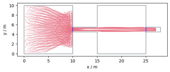
Visualization#

Let’s have a look at the visualization of the simulated trajectories:

from jupedsim.internal.notebook_utils import animate, read_sqlite_file

trajectory_data, walkable_area = read_sqlite_file(trajectory_file)
animate(trajectory_data, walkable_area)

Analysis#

We’ll investigate the \(N-t\) curve and Voronoi density with the help of PedPy.

We evaluate the \(N−t\) curve at the exit for room 1 and room 2. The gradient of this curve provides insights into the flow rate through the bottlenecks. Subsequently, we assess the Voronoi density for the whole geometry. This allows to identify areas in the setup where jamming occurs.

Let’s start with the \(N-t\) curve. We define two measurement lines: between room 1 and the corridor and between room 2 and the corridor. To reuse the measurement lines for the scenario with the wider bottleneck we enlarge it here.

measurement_line1 = pedpy.MeasurementLine([(10, 4.4), (10, 5.6)])
measurement_line2 = pedpy.MeasurementLine([(25, 4.4), (25, 5.6)])

pedpy.plot_measurement_setup(
    walkable_area=walkable_area,
    traj=trajectory_data,
    traj_alpha=0.5,
    traj_width=1,
    measurement_lines=[measurement_line1, measurement_line2],
    ml_color="b",
    ma_line_width=1,
    ma_alpha=0.2,
).set_aspect("equal")

../_images/ad7367413fdeb00d2e581da8344422a2ce8442172f4f47b0c45f585523a41028.png

As a next stept we calculate the \(N-t\) data and plot it:

nt1, crossing_frames1 = pedpy.compute_n_t(
    traj_data=trajectory_data,
    measurement_line=measurement_line1,
)
nt2, crossing_frames2 = pedpy.compute_n_t(
    traj_data=trajectory_data,
    measurement_line=measurement_line2,
)

fig = plt.figure()
ax = fig.add_subplot(111)
ax.set_title("N-t")
ax.plot(
    nt1["time"],
    nt1["cumulative_pedestrians"],
    label="First Bottleneck",
)
ax.plot(nt2["time"], nt2["cumulative_pedestrians"], label="Second Bottleneck")
ax.legend()
ax.set_xlabel("t / s")
ax.set_ylabel("# Pedestrians")
plt.show()

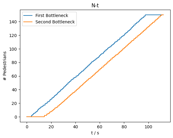
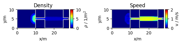
../_images/1ba5045a3ad685d887adac3d5b74cf11dddc2f6d48b584e905358be80a46ed2f.png

The results above show a similar and time-shifted flow for both bottlenecks. Further, to inspect the formation of jamming we analyse the individual speed and density over time. To do so, we use PedPy to calculate the individual speed and Voronoi polygons for each frame calculated by the simulation.

individual_speed = pedpy.compute_individual_speed(
    traj_data=trajectory_data,
    frame_step=5,
    speed_calculation=pedpy.SpeedCalculation.BORDER_SINGLE_SIDED,
)

individual_voronoi_cells = pedpy.compute_individual_voronoi_polygons(
    traj_data=trajectory_data,
    walkable_area=walkable_area,
    cut_off=pedpy.Cutoff(radius=0.8, quad_segments=3),
)

Now we calculate the profiles in a grid of 0.25 x 0.25 meters for the time period in which the agents are entering the first bottleneck. This usually requires a bit of computation time, which is why we only consider 100 frames.

min_frame_profiles = 1800
max_frame_profiles = 1900

density_profiles, speed_profiles = pedpy.compute_profiles(
    individual_voronoi_speed_data=pd.merge(
        individual_voronoi_cells[
            individual_voronoi_cells.frame.between(
                min_frame_profiles, max_frame_profiles
            )
        ],
        individual_speed[
            individual_speed.frame.between(
                min_frame_profiles, max_frame_profiles
            )
        ],
        on=["id", "frame"],
    ),
    walkable_area=walkable_area.polygon,
    grid_size=0.25,
    speed_method=pedpy.SpeedMethod.ARITHMETIC,
)

../_images/6c159a1b3044c731770e242ce00f116ccfbd482ee242a86897c27ecdb3438096.png

Comparison of Different Bottleneck Widths#

As a last step we’ll investigate how the width of the bottleneck influences our results. For this purpose, we’ll configure and run the simulation with the exact same parameters except for the geometry. We will change the width of the corridor to 0.8 and 1.2 meters and compare the results.

Scenario with a Narrower Bottleneck#

Let’s configure the simulation with a corridor width of 0.8 meters. We can reuse most of the parameters from our first simulation.

We define the walkable area:

corridor_narrow = Polygon([(10, 4.6), (28, 4.6), (28, 5.4), (10, 5.4)])
area_narrow = GeometryCollection(corridor_narrow.union(room1.union(room2)))
walkable_area_narrow = pedpy.WalkableArea(area_narrow.geoms[0])
pedpy.plot_walkable_area(walkable_area=walkable_area_narrow).set_aspect("equal")

../_images/fc81a57eb29961325ae9e9533da3a506cfbe9358e47d7a3ac2824472876a6af1.png

The starting positions, exit, operational model parameters and general agent parameter remain the same. So we just need to setup a new simulation object with the journeys:

trajectory_file_narrow = "double-botteleneck_narrow.sqlite"  # output file
simulation_narrow = jps.Simulation(
    model=jps.CollisionFreeSpeedModel(),
    geometry=area_narrow,
    trajectory_writer=jps.SqliteTrajectoryWriter(
        output_file=pathlib.Path(trajectory_file_narrow)
    ),
)

exit_id = simulation_narrow.add_exit_stage(exit_area.exterior.coords[:-1])
journey = jps.JourneyDescription([exit_id])
journey_id = simulation_narrow.add_journey(journey)

And execute the simulation - this may take a bit of computation time since the corridor is quite narrow:

for pos, v0 in zip(pos_in_spawning_area, v_distribution):
    simulation_narrow.add_agent(
        jps.CollisionFreeSpeedModelAgentParameters(
            journey_id=journey_id,
            stage_id=exit_id,
            position=pos,
            desired_speed=v0,
            radius=0.15,
        )
    )

while simulation_narrow.agent_count() > 0:
    simulation_narrow.iterate()

from jupedsim.internal.notebook_utils import animate, read_sqlite_file

trajectory_data_narrow, walkable_area = read_sqlite_file(trajectory_file_narrow)
animate(trajectory_data_narrow, walkable_area)

Scenario with a Wider Bottleneck#

Next, we configure the simulation with a corridor width of 1.2 meters. The steps are the same as for the narrower botteleck:

corridor_wide = Polygon([(10, 4.4), (28, 4.4), (28, 5.6), (10, 5.6)])
area_wide = GeometryCollection(corridor_wide.union(room1.union(room2)))
walkable_area_wide = pedpy.WalkableArea(area_wide.geoms[0])
pedpy.plot_walkable_area(walkable_area=walkable_area_wide).set_aspect("equal")

../_images/24d3b156f0b83eb20ef56dbcebcc55d26c7228790c449386fc0fcdc3a3096b30.png

trajectory_file_wide = "double-botteleneck_wide.sqlite"  # output file
simulation_wide = jps.Simulation(
    model=jps.CollisionFreeSpeedModel(),
    geometry=area_wide,
    trajectory_writer=jps.SqliteTrajectoryWriter(
        output_file=pathlib.Path(trajectory_file_wide)
    ),
)

exit_id = simulation_wide.add_exit_stage(exit_area.exterior.coords[:-1])
journey = jps.JourneyDescription([exit_id])
journey_id = simulation_wide.add_journey(journey)

for pos, v0 in zip(pos_in_spawning_area, v_distribution):
    simulation_wide.add_agent(
        jps.CollisionFreeSpeedModelAgentParameters(
            journey_id=journey_id,
            stage_id=exit_id,
            position=pos,
            desired_speed=v0,
            radius=0.15,
        )
    )

while simulation_wide.agent_count() > 0:
    simulation_wide.iterate()

from jupedsim.internal.notebook_utils import animate, read_sqlite_file

trajectory_data_wide, walkable_area = read_sqlite_file(trajectory_file_wide)
animate(trajectory_data_wide, walkable_area)

Comparison of the Results#

Now we can compare the \(N-t\) curves for the three scenarios.

nt1_narrow, crossing_frames1_narrow = pedpy.compute_n_t(
    traj_data=trajectory_data_narrow,
    measurement_line=measurement_line1,
)
nt1_wide, crossing_frames1_wide = pedpy.compute_n_t(
    traj_data=trajectory_data_wide,
    measurement_line=measurement_line1,
)

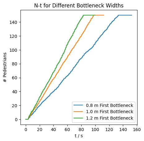
../_images/2976a70cff9a06d71bc1c082f6ea37e7e29bfda1cc3ef30874e1c19dbe111e86.png

The results show: the smaller the width of the bottleneck, the smaller the flow as it takes longer for all 150 agents to enter the first bottleneck.

Download#