How to work with Journeys

This notebook can be directly downloaded here to run it locally.

With JuPedSim, directing agents towards exits and ensuring a smooth evacuation from the simulation area is straightforward and versatile. There might be scenarios where it’s vital to navigate agents along various paths, thus creating diverse evacuation situations. Let’s explore different routing strategies of agents using a simple geometric space - a corner.

JuPedSim manages routing by geometrically triangulating the simulation area. Without user-defined routing strategies, agents, for example, in a corner simulation, naturally move towards the inner edge of the corner. Look at this visualization where the given direction of each agent is shown by a red line. You’ll observe all red lines lead towards the exit along the inner edge of the corner. While it seems logical, this path isn’t always optimal and could result in a bottleneck, thereby slowing down the evacuation process.

Show code cell source Hide code cell source

import pathlib

import jupedsim as jps
import matplotlib.pyplot as plt
import numpy as np
import pedpy
from matplotlib.patches import Circle
from shapely import Polygon

%matplotlib inline

Preparing the Simulation: Geometry and Routing Instructions

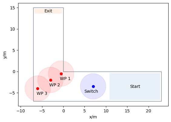
Let’s start by setting up a basic polygon. This will serve as our main simulation area where agents will be distributed. Additionally, we’ll mark an exit area using another polygon. When agents enter this exit area, they’re deemed to have safely evacuated and will be removed from the ongoing simulation.

Next, we’ll introduce an initial target for the agents: a sizable circular area (known as a switch). After the simulation kickstarts, agents will first head towards this circle. Once they enter the circle, they’ll be directed to one of three distinct waypoints, set diagonally along the curve of the corner.

For the simulation’s onset, all agents will be positioned inside a rectangular zone at the corner’s base.

simulation_polygon = Polygon(
    [(-7, 15), (-7, -7), (23, -7), (23, 0), (0, 0), (0, 15)]
)
exit_polygon = [(-6.8, 14.8), (-0.2, 14.8), (-0.2, 13.5), (-6.8, 13.5)]
switch_point = (7, -3.5)
waypoints = [
    (-0.5, -0.5),
    (-3, -2),
    (-6, -4),
]
distance_to_waypoints = 3
distance_to_switch = 3

distribution_polygon = Polygon(
    [[22.8, -0.3], [10.8, -0.3], [10.8, -6.8], [22.8, -6.8]]
)
walkable_area = pedpy.WalkableArea(simulation_polygon)

Show code cell source Hide code cell source

fig, ax = plt.subplots(nrows=1, ncols=1)
ax.set_aspect("equal")
pedpy.plot_walkable_area(walkable_area=walkable_area, axes=ax)

x, y = distribution_polygon.exterior.xy
plt.fill(x, y, alpha=0.1)
plt.plot(x, y, color="white")
centroid = distribution_polygon.centroid
plt.text(centroid.x, centroid.y, "Start", ha="center", va="center", fontsize=10)

x, y = Polygon(exit_polygon).exterior.xy
plt.fill(x, y, alpha=0.1)
plt.plot(x, y, color="white")
centroid = Polygon(exit_polygon).centroid
plt.text(centroid.x, centroid.y, "Exit", ha="center", va="center", fontsize=10)

ax.plot(switch_point[0], switch_point[1], "bo")
circle = Circle(
    (switch_point[0], switch_point[1]),
    distance_to_switch,
    fc="blue",
    ec="blue",
    alpha=0.1,
)
ax.add_patch(circle)
ax.annotate(
    "Switch",
    (switch_point[0], switch_point[1]),
    textcoords="offset points",
    xytext=(-5, -15),
    ha="center",
)
for idx, waypoint in enumerate(waypoints):
    ax.plot(waypoint[0], waypoint[1], "ro")
    ax.annotate(
        f"WP {idx+1}",
        (waypoint[0], waypoint[1]),
        textcoords="offset points",
        xytext=(10, -15),
        ha="center",
    )
    circle = Circle(
        (waypoint[0], waypoint[1]),
        distance_to_waypoints,
        fc="red",
        ec="red",
        alpha=0.1,
    )
    ax.add_patch(circle)

num_agents = 100
positions = jps.distribute_by_number(
    polygon=distribution_polygon,
    number_of_agents=num_agents,
    distance_to_agents=0.4,
    seed=12,
    distance_to_polygon=0.2,
)

Exploring Transition Strategies

All agents initially set their course towards the switch_point. After reaching it, they navigate towards intermediate goals (waypoints) before making their way to the final exit. The challenge lies in deciding which waypoint each agent should target next.

Let’s explore three unique methods to determine these transition strategies:

1. Direct Path Strategy: Here, every agent simply aims for the first waypoint, mirroring a shortest path algorithm.

2. Balanced Load Strategy: Agents are directed towards the least occupied waypoint, ensuring a more balanced distribution.

3. Round Robin Strategy: Waypoints are sequentially assigned to agents, rotating through each in turn.

---

Direct Path Strategy

def shortest_path(simulation: jps.Simulation, switch_id, waypoint_ids, exit_id):
    """Build a journey with fixed transitions for a given simulation."""

    journey = jps.JourneyDescription([switch_id, *waypoint_ids, exit_id])
    # switch ---> 1st waypoint
    journey.set_transition_for_stage(
        switch_id, jps.Transition.create_fixed_transition(waypoint_ids[0])
    )
    # 1st waypoint ---> exit
    journey.set_transition_for_stage(
        waypoint_ids[0], jps.Transition.create_fixed_transition(exit_id)
    )

    journey_id = simulation.add_journey(journey)
    return journey_id

Balanced Load Strategy

def least_targeted(
    simulation: jps.Simulation, switch_id, waypoint_ids, exit_id
):
    """Build a journey with least targeted transitions for a given simulation."""

    journey = jps.JourneyDescription([switch_id, *waypoint_ids, exit_id])
    # switch ---> least targeted waypoint
    journey.set_transition_for_stage(
        switch_id,
        jps.Transition.create_least_targeted_transition(waypoint_ids),
    )
    # from all waypoints ---> exit
    for waypoint_id in waypoint_ids:
        journey.set_transition_for_stage(
            waypoint_id, jps.Transition.create_fixed_transition(exit_id)
        )

    journey_id = simulation.add_journey(journey)
    return journey_id

Round Robin Strategy

def round_robin(simulation: jps.Simulation, switch_id, waypoint_ids, exit_id):
    """Build a journey with least round-robin transitions for a given simulation."""

    journey = jps.JourneyDescription([switch_id, *waypoint_ids, exit_id])
    # switch ---> 1st waypoint with weight1
    # switch ---> 2nd waypoint with weight2
    # switch ---> 3th waypoint with weight3
    weight1, weight2, weight3 = 1, 1, 1
    journey.set_transition_for_stage(
        switch_id,
        jps.Transition.create_round_robin_transition(
            [
                (waypoint_ids[0], weight1),
                (waypoint_ids[1], weight2),
                (waypoint_ids[2], weight3),
            ]
        ),
    )
    # from all waypoints ---> exit
    for waypoint_id in waypoint_ids:
        journey.set_transition_for_stage(
            waypoint_id, jps.Transition.create_fixed_transition(exit_id)
        )

    journey_id = simulation.add_journey(journey)
    return journey_id

scenarios = [
    shortest_path,
    least_targeted,
    round_robin,
]

Executing the Simulation

With all components in place, we’re set to initiate the simulation. For this demonstration, the trajectories will be recorded in an sqlite database.

First we setup some agent parameters then run three simulation with the different strategies:

def run_scenario_simulation(scenario, agent_parameters, positions, geometry):
    """Runs a simulation for a given scenario using the provided simulation object, agent parameters, and positions."""
    filename = f"{scenario.__name__}.sqlite"

    simulation = jps.Simulation(
        dt=0.05,
        model=jps.CollisionFreeSpeedModel(
            strength_neighbor_repulsion=2.6,
            range_neighbor_repulsion=0.1,
            range_geometry_repulsion=0.05,
        ),
        geometry=geometry,
        trajectory_writer=jps.SqliteTrajectoryWriter(
            output_file=pathlib.Path(filename)
        ),
    )
    exit_id = simulation.add_exit_stage(exit_polygon)
    switch_id = simulation.add_waypoint_stage(switch_point, distance_to_switch)
    waypoint_ids = [
        simulation.add_waypoint_stage(waypoint, distance_to_waypoints)
        for waypoint in waypoints
    ]
    agent_parameters.stage_id = switch_id
    journey_id = scenario(simulation, switch_id, waypoint_ids, exit_id)
    agent_parameters.journey_id = journey_id
    for new_pos in positions:
        agent_parameters.position = new_pos
        simulation.add_agent(agent_parameters)

    while simulation.agent_count() > 0:
        simulation.iterate()

    return filename, simulation.iteration_count()

for scenario in scenarios:
    filename, iteration_count = run_scenario_simulation(
        scenario,
        jps.CollisionFreeSpeedModelAgentParameters(),
        positions,
        walkable_area.polygon,
    )

Visualizing the Trajectories

To visualize trajectories, we’ll pull simulation data from the SQLite database and then employ a helper function to depict the agent movements. For subsequent analyses, we’ll organize these trajectory files within a dictionary for easy access.

from jupedsim.internal.notebook_utils import animate, read_sqlite_file

agent_trajectories = {}
for scenario in scenarios:
    scenario_name = scenario.__name__
    agent_trajectories[scenario_name], walkable_area = read_sqlite_file(
        f"{scenario_name}.sqlite"
    )
    animate(
        agent_trajectories[scenario_name],
        walkable_area,
        title_note=f"Scenario: {scenario_name}",
        every_nth_frame=10,
    ).show()

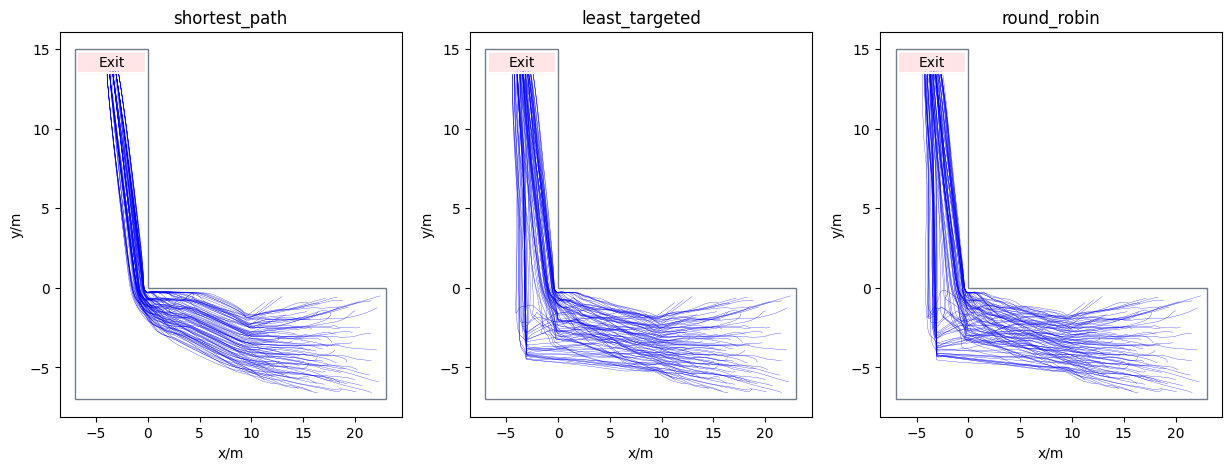
Analysis of the results

With three distinct evacuation simulations completed, it’s time to dive into the outcomes. Let’s start by visualizing the trajectories. This will give us an initial insight into the variations among the scenarios:

fig, axes = plt.subplots(nrows=1, ncols=3, figsize=(15, 5))
for name, ax in zip(agent_trajectories, axes):
    pedpy.plot_trajectories(
        traj=agent_trajectories[name],
        walkable_area=walkable_area,
        axes=ax,
        traj_width=0.2,
        traj_color="blue",
    )
    x, y = Polygon(exit_polygon).exterior.xy
    ax.fill(x, y, alpha=0.1, color="red")
    ax.plot(x, y, color="white")
    centroid = Polygon(exit_polygon).centroid
    ax.text(
        centroid.x, centroid.y, "Exit", ha="center", va="center", fontsize=10
    )
    ax.set_title(name)

Calculate profiles

from typing import Tuple

import numpy.typing as npt
from scipy import stats


def calculate_density_average_classic(
    bounds: Tuple[float, float, float, float],
    dx: float,
    nframes: int,
    X: npt.NDArray[np.float64],
    Y: npt.NDArray[np.float64],
) -> npt.NDArray[np.float64]:
    """Calculate classical method

    Density = mean_time(N/A_i)
    """
    geominX, geominY, geomaxX, geomaxY = bounds
    xbins = np.arange(geominX, geomaxX + dx, dx)
    ybins = np.arange(geominY, geomaxY + dx, dx)
    area = dx * dx
    ret = stats.binned_statistic_2d(
        X,
        Y,
        None,
        "count",
        bins=[xbins, ybins],
    )
    return np.array(np.nan_to_num(ret.statistic.T)) / nframes / area

Show code cell source Hide code cell source

from plotly.subplots import make_subplots


def plot_classical_density_profile(data, walkable_area, name, dx, rho_max):
    geominX, geominY, geomaxX, geomaxY = walkable_area.bounds
    title = f"<b>{name}</b>"
    fig = make_subplots(rows=1, cols=1, subplot_titles=([title]))
    xbins = np.arange(geominX, geomaxX + dx, dx)
    ybins = np.arange(geominY, geomaxY + dx, dx)
    x, y = walkable_area.polygon.exterior.xy
    x = list(x)
    y = list(y)
    heatmap = go.Heatmap(
        x=xbins,
        y=ybins,
        z=data,
        zmin=0,
        zmax=rho_max,
        name=title,
        connectgaps=False,
        zsmooth=None,
        hovertemplate="Density: %{z:.2f}<br>\nPos: (%{x:2f}: %{y:.2f}}",
        colorbar=dict(title="Density"),
        colorscale="Jet",
    )
    fig.add_trace(heatmap)
    #    Geometry walls
    line = go.Scatter(
        x=x,
        y=y,
        mode="lines",
        name="wall",
        showlegend=False,
        line=dict(
            width=3,
            color="white",
        ),
    )
    fig.add_trace(line)

    return fig

Show code cell source Hide code cell source

import math

import plotly.graph_objects as go

dx = 0.5
rho_max = -1
fig = make_subplots(
    rows=1, cols=3, subplot_titles=(list(agent_trajectories.keys()))
)
for count, name in enumerate(agent_trajectories):
    trajectories = agent_trajectories[name]
    data = calculate_density_average_classic(
        walkable_area.bounds,
        dx,
        nframes=trajectories.data["frame"].max(),
        X=trajectories.data["x"],
        Y=trajectories.data["y"],
    )
    rho_max = max(np.max(data), rho_max)
    ind_fig = plot_classical_density_profile(
        data, walkable_area, name, dx, math.ceil(rho_max)
    )
    for trace in ind_fig.data:
        fig.add_trace(trace, row=1, col=count + 1)

    fig.update_xaxes(title_text="X [m]", row=1, col=count + 1)
    fig.update_yaxes(title_text="Y [m]", scaleanchor="x", scaleratio=1)
fig

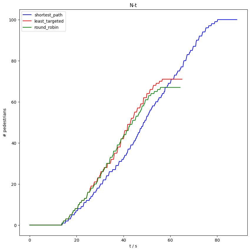
Analyzing Evacuation Duration

To further understand our earlier observations, we compute the \(N−t\) diagram, which shows when an agent crosses a designated measurement line. We position this line near the exit and evaluate the \(N−t\) curves for all three simulations, subsequently determining the respective evacuation durations.

Note: It’s essential to position the measurement line inside the simulation area, ensuring that agents cross it.

import warnings

warnings.filterwarnings("ignore")
measurement_line = pedpy.MeasurementLine([[-3, 4], [0, 4]])
fig, ax = plt.subplots(nrows=1, ncols=1, figsize=(10, 10))
colors = ["blue", "red", "green"]
for i, name in enumerate(agent_trajectories):
    nt, _ = pedpy.compute_n_t(
        traj_data=agent_trajectories[name],
        measurement_line=measurement_line,
    )
    ax = pedpy.plot_nt(nt=nt, color=colors[i])
    ax.lines[-1].set_label(name)
    Time = np.max(nt["time"])
    print(
        "Name: {:<20} Evacuation time: {:<15}".format(
            name, "{} seconds".format(Time)
        )
    )
ax.legend()
plt.show()

Name: shortest_path        Evacuation time: 88.4 seconds   
Name: least_targeted       Evacuation time: 65.0 seconds   
Name: round_robin          Evacuation time: 64.2 seconds   

Findings and Conclusions

The exploration of density profiles demonstrates notable variations in agent distribution, contingent upon the algorithm employed. The shortest path algorithm, aligning with our initial predictions, induces higher densities prior to encountering the corner. Conversely, the round-robin algorithm demonstrates a capacity to redistribute the jam, steering agents away from the corner bend and facilitating a more even spread around it.

A vital observation from the simulations underscores the role of waypoint placement, particularly when positioned as circles, along with the discernment of their range. This cruciality not only impacts agent navigation but also influences the effectiveness of the deployed algorithm.

Future Considerations

As the waypoint placement proves to be instrumental, ensuing studies or simulations might delve into optimizing these placements, exploring a range of scenarios and algorithmic strategies to discern optimal configurations for various contexts. Furthermore, additional research could investigate the scalability of these findings, examining the consistency of agent distribution patterns in scenarios with varying agent quantities, environmental layouts, and navigational complexities.

Download

This notebook can be directly downloaded here to run it locally.